Deep dive

Building Sonic: an implicit-feedback recommender, end to end

August 2026 · updated · 19 min · Live demo · API · Code on GitHub

Sonic recommends musical artists from Last.fm listening history. That sentence describes a hundred tutorials, so this post is about the parts the tutorials skip: what implicit feedback changes about the problem, why the evaluation harness got built before the model, and what happened when I scaled to real data and the whole thing inverted. The tuned ALS model I spent most of the project on is not the model that ships. Getting there taught me more than the tuning did.

1. The data, and why it's mostly holes

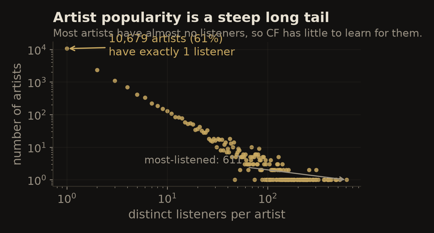
The input is a user-artist-playcount table: who listened to whom, and how often. Turned into a matrix with users as rows and artists as columns, it is almost entirely empty. That emptiness is the defining property of the problem, not an inconvenience on the way to it, and every design decision downstream traces back to it.

Listening also follows a brutal power law. A small set of artists absorbs an enormous share of plays while the long tail collects a handful each, and individual users are just as lopsided. Any model fit on raw playcounts without accounting for this learns that everyone should listen to the most-played artists. Technically correct, completely useless.

The starting dataset was Last.fm HetRec 2011: 1,892 users, 17,632 artists, 92,834 listening records, 99.72% empty. Hold onto one detail, because section six turns on it. Every user in that file is truncated to roughly their top fifty artists. It is not a record of what people listened to; it is a record of what people listened to most, which is a different and much easier thing to predict.

2. Implicit feedback and confidence weighting

Nobody rates artists on Last.fm. There are no stars, no thumbs, only behavior, and behavior is ambiguous in a way ratings are not. A one-star rating is information: this user tried it and disliked it. A zero playcount is two very different things wearing the same mask, since the user may have heard the artist and rejected them, or may never have encountered them at all, and nothing in the matrix distinguishes the cases.

The implicit ALS formulation splits the signal in two: a binary preference (did any interaction happen) and a confidence weight derived from its magnitude.

preference  p_ui = 1 if playcount > 0 else 0
confidence  c_ui = 1 + alpha * playcount

Zeros stay in the training objective, but at low confidence, which is exactly the right treatment of an ambiguous signal, since they still say something, just quietly. Meanwhile a user who played an artist two hundred times contributes a strongly-weighted positive. alpha is the dial between treating heavy listening as mild interest versus overwhelming proof, and it matters more than people expect.

One preprocessing decision cuts against instinct. Counts here span 1 to 352,698, six orders of magnitude, so passing them in untransformed lets a handful of superfans dictate the latent space. Compressing the scale first keeps the heaviest listeners influential without letting them run the factorization, so the formula becomes c = 1 + alpha * log(1 + count). The ablation is unambiguous: with raw counts ALS peaks at 0.098 NDCG@10 and degrades to 0.024 as alpha rises; with log-scaled counts it reaches 0.158 and stays strong across the whole range.

All of this is machinery the shipped model does not use. I'm leaving it in because it was load-bearing for most of the project, and because the reason it got abandoned is the interesting part.

3. The evaluation harness, written first

Before any factorization ran, the grader existed. This ordering is the single most useful decision in the project, because a recommender that has never been scored cannot be tuned, and "these recommendations look reasonable to me" is not a measurement, it is a vibe.

The design: for each user, hide a slice of the artists they actually listened to, hand the model everything else, ask for a ranked top-k, and measure how much of the hidden truth comes back. Simple to state, and full of decisions once you write it yourself: users too sparse to split at all, masking already-seen artists out of the candidate list, deterministic tie handling so the same model doesn't score differently across runs, and the fact that recall@10 is capped below 1.0 by construction whenever a user's hidden set exceeds ten. Three metrics came out of it: precision@k for list purity, recall@k for how much of the hidden set surfaced, and NDCG for position.

The split needed the same care. A random split of interaction rows leaks: to recommend for a user the model must learn their vector from training interactions, and a row split quietly drops held-out artists into that vector and inflates the score. Splitting whole users into a test group fails the opposite way, with no vector at all, so you measure the cold-start fallback instead of the recommender. The harness holds out a fraction of each user's interactions and keeps the rest of their history in train.

Two pieces of structure enforce that rather than asking for it. The metrics and split live in one file the tuning loop cannot edit, on the theory that if the thing trying to win can rewrite the rules of winning, the search is unfalsifiable. And a slice of data was sealed into a locked holdout whose path is defined only in the one-time split script, so the loop has no symbol pointing at it. It was read exactly once, at the end: NDCG@10 = 0.233 ± 0.001, slightly above the cross-validated score thanks to the extra training data, with no sign of overfitting.

4. The baseline that refuses to lose

Recommend the globally most-played artists to everyone. No personalization, no model, no latent factors. That baseline is embarrassingly strong here for a structural reason: when listening concentrates this heavily, the popular artists genuinely are the ones most users have heard, so the list scores real hits on real holdout sets. Hence a standing rule: a model counts only if it beats popularity on the identical harness and split.

Measured that way, tuned ALS reached precision@10 of 0.132 against popularity's 0.050, and NDCG@10 of 0.171 against 0.063, roughly 2.7× on both across 1,883 scored users. Not split noise, either: a paired user-level bootstrap puts the NDCG@10 difference at +0.108, 95% CI [0.101, 0.115], p < 0.001, with ALS ahead for 63% of users individually.

And that is where most write-ups stop, which is the problem. Ferrari Dacrema and colleagues made the point sharply in 2019: recommender papers routinely beat weak baselines, skip the significance test, and report progress that evaporates when someone tries a well-tuned simple method. Popularity is a weak baseline. Clearing it proves the model does something, not that it does something worth the complexity. So the comparison included two harder opponents: item-item BM25, a neighbourhood model with no factorization at all, at 0.144, and BPR at 0.119. ALS's real margin is the one over BM25: +0.027 NDCG@10, 95% CI [0.021, 0.034], p < 0.001. Significant, and considerably less impressive than 2.7×. That is the honest version.

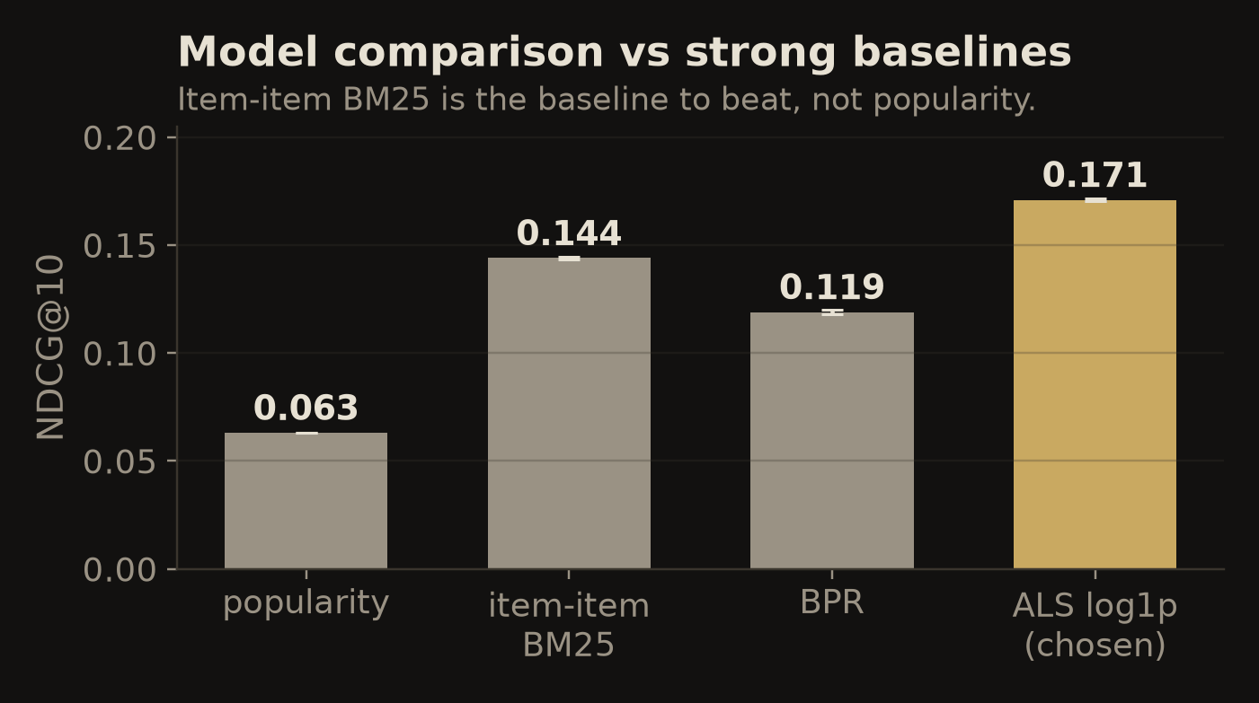
The per-user view is more uncomfortable still. ALS beats BM25 on average but wins for only 46% of users, loses for 30%, and ties for 24%, much of that mass being users where both models simply miss, because at this sparsity many users are hard for anything. A win of that shape argues for routing between the two, not for declaring one correct.

5. The sweep, and the conclusion it reached too early

Four knobs. Latent factors set the dimensionality of the taste space. Too few and distinct genres collapse together, too many and the model memorizes noise in the tail, where most users live. Regularization is the counterweight, and the tail is nothing but sparse rows. Alpha is the confidence scaling from section two, the least intuitive of the four. Iterations are cheap to raise and quick to plateau.

Twelve configurations, pre-registered before the run, three seeds each, every one graded by the identical frozen harness on the identical split. That constraint is what makes a sweep mean anything: if the evaluation drifts between runs, the winner might just be whichever config got graded on the easiest exam.

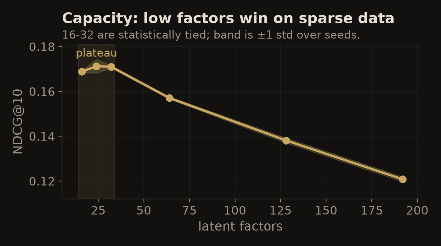
Two results, one of them a trap. The honest one is about picking from a plateau: the nominal winner was 24 factors at 0.1712, but 32 scored 0.1710 with a seed band roughly five times tighter. Overlapping bands mean no real difference, so the tiebreak goes to the stabler configuration rather than the one whose point estimate sits a thousandth higher. Taking the nominal maximum off a noisy plateau is how you end up tuning to a seed.

The trap was the headline. Low capacity wins, complexity does not pay, sparse data cannot support a bigger model. Clean, satisfying, well-supported. A deep Mult-VAE, tried later, came in behind everything. Every number backed the story, and the story was about the wrong thing. It was not a fact about music recommendation. It was a fact about a dataset where every user had been clipped to fifty artists.

6. The pivot: real data, and the ranking flips

Two things had gone wrong, tangled together. The first was the split: sealing 20% into the locked holdout and then holding out another 20% for test left only about 64% of each user's history to train on. On data this thin that is not a rounding error. It alone dropped NDCG@10 from 0.23 to 0.17. Re-cut to 10% holdout and roughly 13.5% test, and a chunk of the deficit disappeared. I had spent real time tuning a model that was mostly being starved.

The second mattered more. The top-fifty cap is not a quirk, it is a different task: predicting a user's favourites from their other favourites, on a matrix where 61% of artists have exactly one listener. So I moved to Last.fm-360K: real, uncapped histories, 17.6M interactions, filtered to a recommendable core of 39,499 users and 11,607 artists with 1.68M interactions. The harness, the metrics, the split logic, the model zoo: all unchanged. Only the data underneath moved.

The ranking flipped.

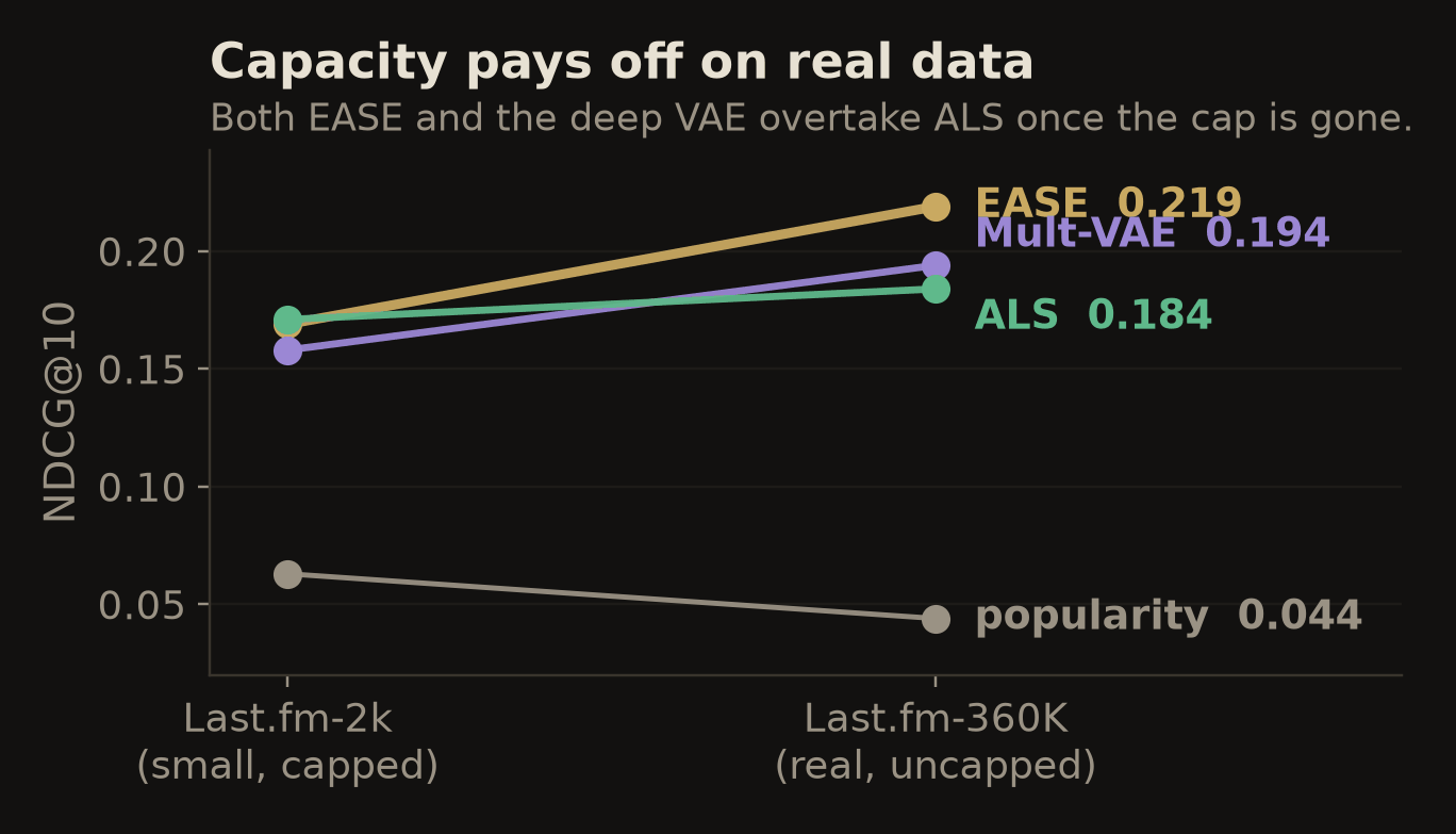
The winner is EASE, a linear item-item autoencoder from Steck (2019), and it is almost aggressively simple. No gradient descent, no epochs, no seeds. Take the item-item Gram matrix, add a ridge term to the diagonal, invert it once, normalize, and zero the diagonal so no item can predict itself. That closed form is the training: one matrix inversion, cubic in the item count, about a minute at this scale, and fully deterministic, which means it has no seed variance to report because it has no seeds.

Final standings on the 360K split, full-catalogue ranking with no sampled shortcuts:

Model	NDCG@10	Recall@10	Coverage
EASE (served)	0.219	0.194	0.42
Mult-VAE (deep)	0.194	0.178	0.81
ALS (128 factors)	0.184	0.163	0.19
item-item BM25	0.110	0.102	0.09
popularity	0.044	0.039	0.00

Every gap is significant under the same paired bootstrap: EASE over Mult-VAE by +0.026, Mult-VAE over ALS by +0.010, EASE over ALS by +0.036, all p < 0.001.

The deep model is the interesting one. Mult-VAE finished last on 2k and second here, overtaking a tuned ALS. Capacity does pay off, it just needs enough data to pay off with, which is precisely what the earlier sweep could not have discovered. And the linear model still won. Both halves are worth holding at once: the small-data result was wrong about complexity, and the fashionable answer still lost to a closed-form ridge regression.

7. Is 0.22 any good?

NDCG@10 of 0.219 does not look like a win, and my instinct was that something was still broken. That instinct is worth interrogating rather than acting on, because a metric has no meaning until you know what scale it lives on.

Two things make the number look small. Every model here ranks the full catalogue, all 11,607 artists, rather than scoring the true item against a sampled handful of negatives, a common shortcut that inflates results substantially. And @10 is a punishing cutoff when a user has dozens of held-out artists. The literature mostly reports @20, @50 and @100; measured there, the same model gives NDCG@100 = 0.361 and Recall@50 = 0.423.

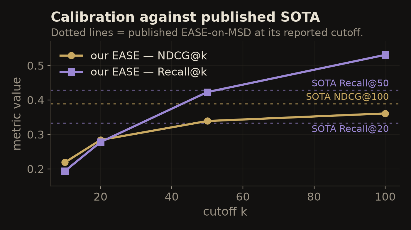
So the model lands in the published band on a comparable dataset. Not beating it, and I am not claiming otherwise, but close enough that the low @10 reading was a cutoff artifact rather than a defect. The temptation when 0.219 first appeared was to go tune something; a five-minute literature check would have saved that instinct a lot of motion. The whole curve gets reported now, so @10 is never seen alone.

8. Coverage doesn't buy accuracy

Accuracy is not the only axis, and the 360K run measured the others: what fraction of the catalogue a model ever recommends, how obscure its picks are, how concentrated its output is. Not decoration: a recommender can score well and still be handing the same three hundred artists to everyone.

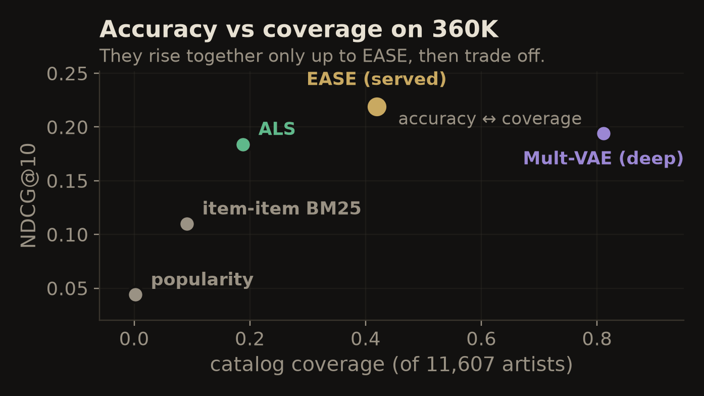
That plot answers a question I had been assuming the answer to. Below EASE, breadth and accuracy improve together, so a narrow model is simply a worse model. Past EASE they trade off, and Mult-VAE's 81% reach against EASE's 42% costs it real accuracy. Wider is not automatically better; the frontier has a corner rather than a slope.

Which makes "how much discovery do you want" a product question with no defensible technical answer, so the API declines to hard-code one. A diversity parameter re-ranks a wider candidate pool with MMR, trading a little relevance for a more varied list, and the caller picks the operating point. Shipping the lever rather than the opinion is the honest move when the data does not tell you where to sit.

9. Cold start, for users and for artists

Collaborative filtering has nothing to say about a user with no interactions. No row to factorize, no neighbours to borrow from, no vector to compute, and a system that returns an error or an empty list in that state is not finished. For unknown users the fallback is popularity, ranked by distinct listeners rather than total plays so one obsessive fan cannot manufacture a hit. It is a genuinely worse recommendation than a user with history gets, and it is the correct trade, because the alternative is none at all.

The more interesting cold-start problem is on the other axis, and I had it backwards for a while. Cold artists are the real gap: with 61% of the catalogue carrying a single listener, no amount of collaborative filtering fixes an item nobody has co-listened. Tags do. A TF-IDF profile over user-applied tags, compared by cosine, needs no listening data whatsoever. 69% of that catalogue carried at least one tag, and tag similarity served 48% of single-listener artists, roughly half the region CF cannot reach. Routing on data availability, co-listening when warm and tags when cold, is a one-line policy and a sensible "fans also like" across the whole catalogue. One caveat: that is a Phase 1 result. The 360K data ships no tags, so the current API's "fans also like" runs on EASE's item-item weights instead.

10. Serving it

The model is exposed through a FastAPI service that takes a user and returns ranked recommendations as JSON. Small amount of code, large amount of the point: a model that only runs inside the notebook that trained it is an experiment, while a model behind an HTTP endpoint is something else can be built on, and serving it forces you to answer questions the notebook lets you dodge.

Those answers turned out to have real design content. The response carries an explicit strategy field: ease, ease+mmr, or cold_start_popularity, because a caller that cannot tell a personalized result from a fallback will silently report fallback traffic as model performance. IDs are matrix indices rather than the source dataset's opaque hashes, which is the only reason the 2k-to-360K pivot did not break every consumer. EASE's weight matrix is not fitted by the service at all. Inverting the 11,607×11,607 Gram matrix is about 10¹² floating-point operations, measured at 85 to 100 s and a 2.5 to 3 GB peak, which would exhaust the container it is supposed to boot. So the fitted 514 MiB matrix is published as a versioned artifact and fetched at startup, with its size and SHA-256 verified before use. A mismatch fails the boot rather than quietly serving the wrong weights. Loading it costs 0.1 s. And a small ALS model is still trained alongside it, not to recommend anything, but to supply the item embeddings MMR needs to measure how similar two candidates are. The tuned model from Phase 1 survives in the served system as a geometry provider.

The same inference core backs a Streamlit app and a written report, so the demo, the service, and the published numbers cannot drift apart.

11. What I'd do differently

Interrogate the dataset's shape before building on it. The top-fifty cap was documented, I read it, and I still treated the data as a given and moved on to modeling. A histogram of interactions per user shows a hard wall at fifty, which is not what organic listening looks like, and that was available on day one. Everything downstream was rigorous and some of it was answering a question about an artifact.

Calibrate before reacting to an absolute number. Knowing that a strong model scores in the low 0.2s at @10 under full-catalogue ranking was a five-minute literature check that would have saved a stretch of unnecessary suspicion about a number that was fine.

Segment the evaluation by user activity level. One macro average pools heavy users, who are easy, with sparse users, who are the hard case, and it can improve while the sparse users get worse. I have the per-user scores. I built the significance tests on them. I just never cut the headline number by cohort.

Keep the whole scoreboard permanent. Popularity, BM25, the previous best model: every future change should clear all of them again on the same frozen harness, because the moment a comparison stops being reported is the moment nobody can tell whether the added complexity is doing anything.

12. Postscript: what shipping it actually took

Added later. Everything above was written when the model was finished. This is what happened when I tried to put it somewhere other people could reach.

Almost none of the distance between "the model works" and "the model is running" was modelling. Four of the failures are worth writing down, because every one of them was invisible to a passing test suite.

The artifact could not be recomputed. EASE's weight matrix is a dense 11,607×11,607 float32 array, 514 MiB. Fitting it means inverting the Gram matrix, which I measured at 85 to 100 s and a 2.5 to 3 GB peak. A container sized to serve the model comfortably cannot afford to build it: the fit would exhaust the machine it is supposed to boot. So the matrix became a published, versioned artifact, fetched at startup with its size and SHA-256 checked before use. A mismatch fails the boot loudly. The failure I did not want is a service that starts happily and serves subtly wrong weights.

The health check was lying. It returned 200 {"status": "ok"} the moment the process was up, while the model was still loading and every recommendation endpoint would have failed. Any orchestrator reads that as "send traffic". A liveness check answers whether the process is alive. A readiness check answers whether it can do the job, and only the second one is useful here. It now returns 503 with a Retry-After until the model is genuinely resident.

The image built fine and the app died on import. First deploy crash-looped on ImportError: libgomp.so.1. The recommendation library ships a compiled extension that opens the OpenMP runtime at import time. The wheel needs no compiler, but it does need a system library that is not in the slim Python base image. Nothing in a normal test run touches that, because the tests pass on a machine that happens to have it. The fix was one line. The lesson was the CI job. The pipeline now builds the container and runs import inside it, which reproduces exactly that failure.

A localhost default shipped to every visitor. The app's "open the report" link read the URL from an environment variable and fell back to http://localhost:8080. The variable was never set in the deployment, so the live site handed every reader a dead link to their own machine. It had been that way for a while. Defaulting to the production URL and overriding locally makes the common case correct by construction. Doing it the other way round makes the visible case quietly wrong.

The surrounding machinery grew to match. Continuous integration runs the linter, a hermetic test suite that needs no model artifacts, and a container build, on every push and on feature branches rather than only after a pull request exists. Dependency updates arrive as grouped, reviewable pull requests with the base image pinned, because the manifests use floor-only versions and a breaking upstream release would otherwise reach the build unannounced. Every request emits a structured JSON log line with a request id and a duration. None of it is novel. The useful part was working out how much of it a project this size actually needs.

Live: dashboard · API · write-up. Code, evaluation harness, and serving layer: github.com/ChrisJ1751/Sonic-Music-Recommendation-System. Data: Last.fm user-artist listening history.