Model exploration
From a popularity baseline to a deep autoencoder, every model we tried, and why EASE won.
Choosing a recommender is not “pick the fanciest model.” It is a gauntlet: run every serious candidate , from a trivial baseline to a deep neural network, through one frozen harness, and let the numbers, with significance tests, decide. This page is the full journey through the model space, the two models it came down to (EASE and a deep Mult-VAE), and the honest finding at the end.
Why run a gauntlet at all
The instinct on a recommender project is to reach for the most powerful model available. The literature says: don’t. Ferrari Dacrema et al. (RecSys 2019) reproduced a wave of “state-of-the-art” neural recommenders and found most were beaten by well-tuned simple methods that the original papers hadn’t compared against properly. Rendle et al. (2022) made the same point from the other side: a carefully-tuned classic (iALS) matches much of the neural SOTA.
The lesson we took: the honest bar is not “beat popularity”, it is “beat the best simple model.” So every candidate runs the same frozen split, the same full-catalogue ranking, and the same paired significance test. No model gets promoted on vibes.
The contenders
We benchmarked five families, spanning trivial to deep:
| Model | Family | Core idea | Why we tried it |
|---|---|---|---|
| Popularity | non-personalised | recommend the most-listened artists to everyone | the honest floor; sparse data makes it deceptively strong |
| item-item BM25 | neighbourhood | recommend artists co-listened with a user’s history, BM25-weighted | the classic “people who listened to X also listened to Y” |
| ALS / iALS | matrix factorization | learn low-rank user & item vectors from implicit confidence (Hu et al. 2008) | the workhorse of implicit-feedback recsys |
| EASE | linear autoencoder | closed-form item-item weight matrix (Steck 2019) | often SOTA on sparse implicit data, no SGD |
| Mult-VAE | deep generative | multinomial variational autoencoder (Liang et al. 2018) | the standard deep model; maximal capacity |
BPR (Rendle 2009) was also in the Phase-1 gauntlet as a pairwise-ranking baseline. The two that mattered at the end were EASE and Mult-VAE, a linear model and a deep one, so the rest of this page focuses on them.
EASE, in depth
EASE (Embarrassingly Shallow AutoEncoder) is deceptively simple: it learns a single item-item weight matrix B such that a user’s score for every artist is their listening vector times B. The trick is that the optimal B, under a squared-error reconstruction objective with an L2 penalty and a hard “an item can’t predict itself” constraint (diag(B) = 0), has a closed form. No gradient descent, no epochs, no learning-rate search:
\[B = -P\,/\,\operatorname{diag}(P), \qquad P = (X^\top X + \lambda I)^{-1}, \qquad B_{ii} = 0\]
def fit_ease(train, reg=100.0):
    X = (train > 0).astype(np.float32).tocsr()
    gram = np.asarray((X.T @ X).todense(), dtype=np.float32)  # item-item co-occurrence
    gram[np.diag_indices_from(gram)] += reg                   # ridge penalty
    inv = np.linalg.inv(gram)                                  # the one expensive step
    B = inv / (-np.diag(inv))                                  # closed-form solution
    B[np.diag_indices_from(B)] = 0.0                           # no self-recommendation
    return B
Why it’s strong. It captures every pairwise item relationship at once (a dense B, unlike sparse neighbourhood models), it has exactly one hyperparameter (λ), and being closed-form it is perfectly reproducible. On sparse implicit data it is a genuine state-of-the-art contender.
What it costs. Inverting the item-item Gram matrix is O(n_items³); at 11,607 artists that is ~a minute and a few GB, and the resulting B is a dense 538 MB matrix. It scales to tens of thousands of items, not millions, and. Being pure collaborative filtering, it uses no audio or tag features, so it cannot help genuinely cold artists.
The deep model, in depth
Mult-VAE is the natural “maximum capacity” challenger. It is a variational autoencoder with a multinomial likelihood (the right fit for “which items did this user interact with”): an encoder compresses a user’s whole listening vector to a small latent distribution, and a decoder reconstructs a probability over all 11,607 artists. It is trained with SGD and KL-annealing.
- Architecture:
11,607 → 600 → 200 (latent) → 600 → 11,607, dropout 0.5, β-annealed KL (Liang 2018’s recommended setup). - Capacity: ~21M parameters and full non-linearity, orders of magnitude more expressive than EASE’s single linear map.
- The hypothesis going in: on the tiny 2k data the deep model lost (too much capacity, too little signal). With 18× more data on 360K, capacity should finally pay off. Does it overtake EASE?
The experiment
Both models, and the full zoo, ran through the identical protocol (src/exp_deep_360k.py):
- the same per-user 360K split (
test_fraction = 0.2, seed = 0); - full-catalogue ranking (all 11,607 artists, no sampled negatives);
- accuracy (NDCG/MAP/Recall) and beyond-accuracy (coverage, novelty, Gini) for every model;
- paired user-level bootstrap (5,000 resamples) for every pairwise claim.
What we found
The deep model climbs, but does not take the crown.
| Model | NDCG@10 | MAP@10 | Recall@10 | Catalog coverage | Novelty |
|---|---|---|---|---|---|
| EASE (served) | 0.219 | 0.112 | 0.194 | 0.419 | 5.26 |
| Mult-VAE (deep) | 0.194 | 0.094 | 0.178 | 0.811 | 6.09 |
| ALS (128 factors) | 0.184 | 0.089 | 0.163 | 0.188 | 5.64 |
| item-item BM25 | 0.110 | 0.047 | 0.102 | 0.091 | 3.65 |
| popularity | 0.044 | 0.017 | 0.039 | 0.002 | 3.16 |
Every gap is significant (paired bootstrap, all p < 0.001):
- EASE − Mult-VAE = +0.026 NDCG@10, the linear model beats the deep one on accuracy.
- Mult-VAE − ALS = +0.010: but the deep model, properly trained, overtakes tuned ALS on real data.
- EASE − ALS = +0.036.
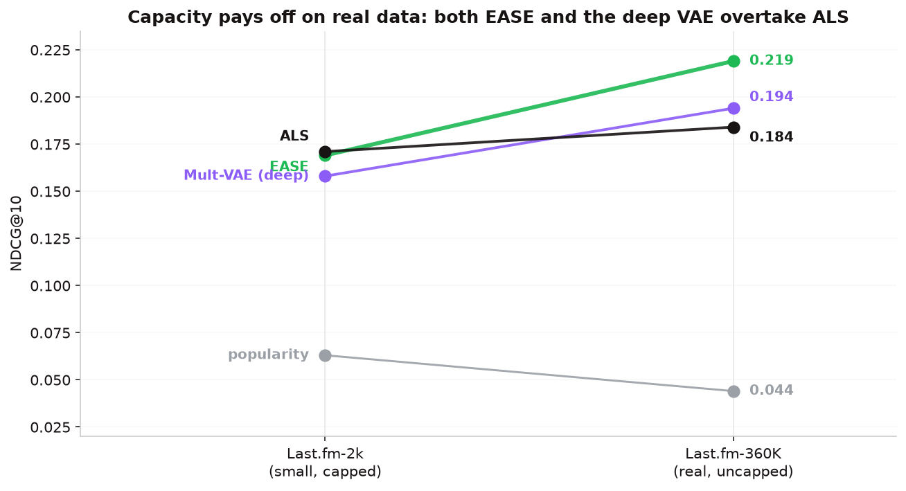
This is the whole arc in one chart. On the small 2k data the deep VAE lost to ALS. On 360K it climbs from last to second. The story is not “deep learning is useless”, it is “deep learning needed the data, and even then the well-designed linear model was better.”
The coverage question, settled
The most tempting intuition on this project was: the deep model covers far more of the catalogue, surely that means higher accuracy too? It is worth settling with the actual numbers, because the answer is “right up to a point, then no.”
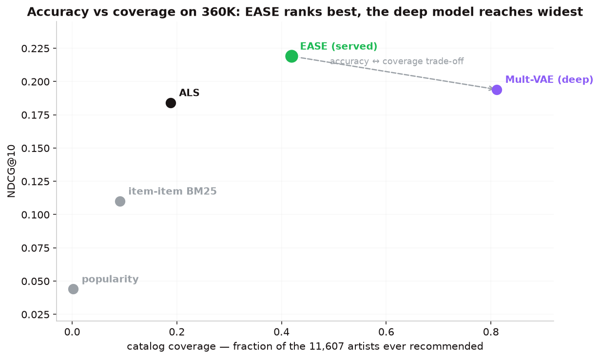
Read the curve left to right. From popularity → BM25 → ALS → EASE, coverage climbs (0.00 → 0.42) and so does accuracy (0.04 → 0.22): a smarter model genuinely reaches more of the catalogue and ranks better. The intuition holds in this regime. But past EASE it turns over, Mult-VAE nearly doubles coverage (0.42 → 0.81) while accuracy falls (0.219 → 0.194).
The mechanism: every user still gets exactly 10 slots. Raising coverage means filling those slots with rarer artists, and a rarer artist is relevant to fewer people, a lower-probability bet per slot. So you cannot buy accuracy by forcing coverage; the causation runs the other way (a smarter model happens to do both) only until you start trading precision for reach. EASE sits at the sweet spot: a healthy 42% coverage and the best ranking. Mult-VAE is the discovery-oriented alternative, the right pick if catalogue reach matters more than top-10 precision.
Verdict
- Served model: EASE. Best accuracy, significantly, and cheap to serve.
- Runner-up with a job: Mult-VAE. Not the accuracy winner, but a legitimate discovery engine (2× the coverage). The
diversity(MMR) lever in the API lets a product owner slide along that frontier at runtime. - The deliverable is the process. A frozen harness trustworthy enough to tell us the deep model was worth trying, that it improved with data, and exactly where it still fell short. With a p-value on every claim.
What we deliberately did not do
Honest scope, and the natural next steps if this were a live product:
- EASE variants: EDLAE (denoising linear autoencoder), higher-order/CEASE, ADMM-SLIM. Sometimes edge out plain EASE by a hair; incremental.
- RecVAE: a stronger VAE than Mult-VAE; the fair “can a better deep model beat EASE?” test.
- iALS done right (Rendle 2022), aggressively-tuned classic MF as the “simple, done properly” angle.
- Hybrid / content features: blend audio and tag signals to reach genuinely cold artists that pure CF cannot, the one place EASE structurally can’t help.
Each is a defensible next experiment; none is likely to change the headline conclusion, which is why we stopped at a crisp, significant result rather than an ever-growing model zoo.
Reproducibility
python -m src.exp_deep_360k     # EASE, ALS, Mult-VAE, popularity on the frozen 360K split
                                # -> outputs/experiments/deep_360k_results.json
Deterministic given seeds. Deep training un-pins the BLAS thread cap (it would be unusably slow at one thread); everything else matches the serving path exactly.