Methodology

Why the numbers are trustworthy.

The point of this project is not a single score, it is a process that produces scores you can believe. Everything below was designed so that no result depends on a lucky seed, a leaked test set, or a weak baseline.

A frozen evaluation harness

Metrics and the data split live in a locked eval_core.py that model code never edits. This is the autoresearch discipline (after Karpathy’s autoresearch pattern): the thing being optimised against must be immovable, or you end up tuning the ruler instead of the model.

Metrics: precision@k, recall@k, NDCG@k, MRR@k, MAP@k. All toy-validated against hand-computed cases in the test suite.
Split ownership: the path to the sealed holdout lives in exactly one file (make_split.py), so no loop or search code even has a symbol pointing at it.

A leakage-safe, per-user holdout

The naive approach, hold out random (user, artist) cells globally. Leaks, because a user’s own held-out listens can inform their training profile. We instead split within each user’s history: part trains, part is a search-visible test set, and part is a sealed holdout read exactly once at the very end.

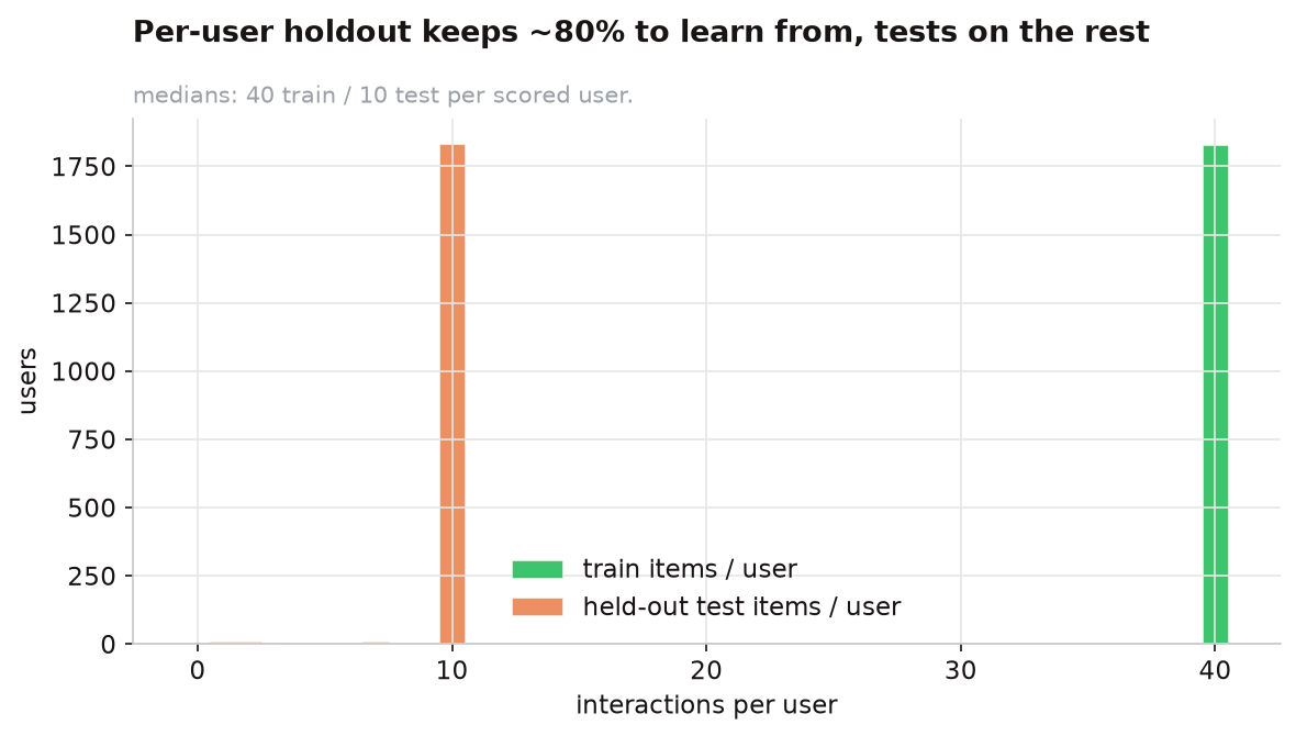
Figure 1: The per-user interaction holdout: each user contributes to train, search-test, and a locked holdout.

The locked holdout was read once, after all model and hyperparameter decisions were final. Every number used to make a decision comes from the search-visible split, never the holdout.

Full-catalogue ranking, not sampled metrics

Every model ranks all 11,607 artists for each user. We deliberately avoid the common shortcut of scoring the true item against a handful of sampled negatives: Krichene & Rendle (KDD 2020) showed that sampled metrics are not just noisier but can re-order which model looks best. Full ranking is more expensive and produces smaller-looking numbers, but they are honest and comparable to the literature.

Strong baselines, not just popularity

Following Ferrari Dacrema et al. (RecSys 2019), who showed that many “state-of-the-art” neural recommenders fail to beat well-tuned simple ones, every model is measured against a real gauntlet: popularity, ALS, BPR, item-item BM25, and a deep Mult-VAE. Beating popularity is table stakes; the honest bar is the best simple method.

Disciplined search (Phase 1)

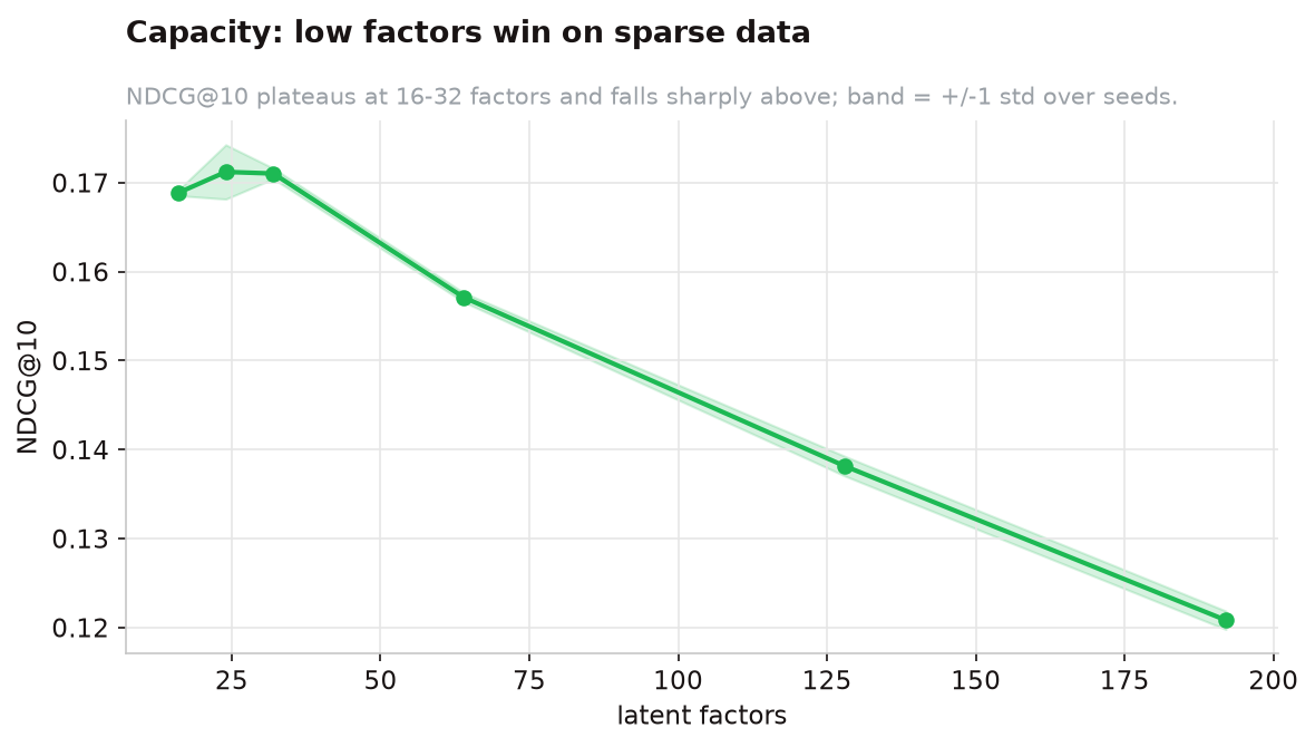
Hyperparameters were chosen by a pre-registered search that logs every configuration to an append-only file and promotes nothing automatically. On the 2k data this is where we learned that capacity was not free, more latent factors did not help.

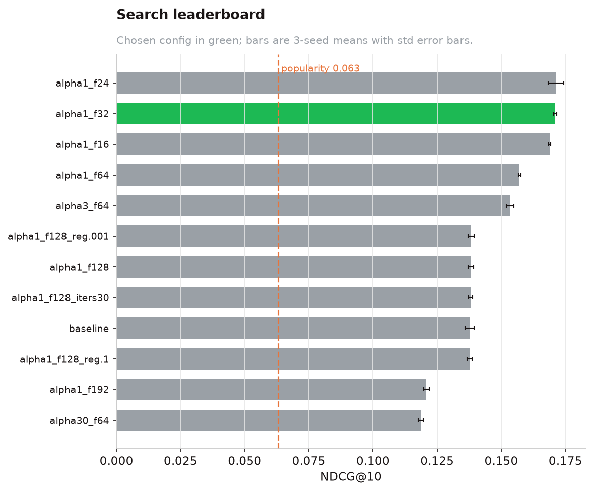
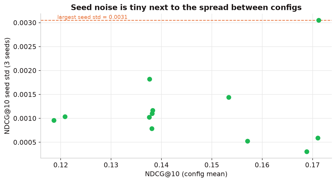
Figure 2: Search leaderboard: configurations ranked on the frozen split.

Figure 3: Factor sweep: low capacity (32 factors) won on the small data.

We also verified seed stability, that the chosen configuration’s ranking was not a fluke of one random seed, rather than importing heavier stability machinery the data did not warrant.

Figure 4: Seed-stability check on the chosen configuration.

Significance, not vibes

Every “X beats Y” claim carries a paired, user-level bootstrap (5,000 resamples) with a confidence interval and a p-value (src/stats.py). A difference in mean NDCG is only reported as real when the interval excludes zero.

How a recommendation is generated

For the served EASE model, a single recommendation request is four steps:

Look up the user’s row in the binarised interaction matrix (what they’ve listened to).
Score every one of the 11,607 artists in one sparse mat-vec: scores = x · B, where B is the learned item-item weight matrix.
Mask the artists the user has already played, so recommendations are genuinely new.
Rank / diversify: take the top-k; if diversity > 0, re-rank a wider pool with MMR (using ALS item embeddings) to trade a little accuracy for a more varied list.

Users with no usable history fall back to a popularity recommender, the safe cold-start path.